A GLOBAL CURVE FIT OF ENZYME KINETICS DATA
A global curve fit is the simultaneous fitting of multiple functions to multiple data sets with possible shared parameters.
There are two types of parameters in the multiple equations:
1. "global" parameters that are estimated from all data sets and
2. "local" parameters which are estimated from individual data sets.
Often there are multiple experiments to determine the Michaelis constant Km and the investigator wants to combine all data in a "global" analysis. In this case you would expect the maximum velocities Vmax to vary across data sets and the Michaelis constant Km to remain the same. The present example from Duggleby (1) globally analyzes nine individual data sets using nine maximum velocity parameters {V1, V2, ..., V9} and one Michaelis constant parameter Km.

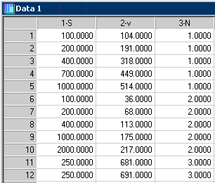
SigmaPlot performs global curve fitting using an index variable to identify the individual data set. The SigmaPlot worksheet below contains a portion of the Duggleby data with the substrate and velocity data in columns 1 and 2, respectively. The index variable is in column 3. It changes across individual data sets from 1 to 9. The index variable is used to associate the velocity parameters with the corresponding data set. For example, it allows the parameter V1 to be determined from the first data set in rows 1 – 5, V2 from the data set in rows 6 – 10, etc. The curve fitter will obtain Km using data from all nine data sets. V1,…, V9 are local parameters and Km is a global parameter.
Use the XYZ curve fit format to analyze the concatenated data set.

The curve fit equations are shown below in the single window dialog format. This dialog is useful when you create your own fit equation. It also allows additional commenting to be viewed.
[Variables]
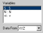
S=col(1) ' substrate data
vi=col(2) ' velocity data
N=col(3) ' index variable data
w=1/vi^2 ' inverse square weighting
[Parameters]
Km = x50(S,vi,0.1)
V1 = max(if(N=1,vi))
V2 = max(if(N=2,vi))
V3 = max(if(N=3,vi))
V4 = max(if(N=4,vi))
V5 = max(if(N=5,vi))
V6 = max(if(N=6,vi))
V7 = max(if(N=7,vi))
V8 = max(if(N=8,vi))
V9 = max(if(N=9,vi))
[Equation]
Vn={V1,V2,V3,V4,V5,V6,V7,V8,V9}[N] ' velocity parameters (indexed by N)
v=Vn/(1 + Km/S) ' Michaelis-Menten equations
fit v to vi with weight w ' fit statement with weighting
[Constraints]
Km>0
[Options]
iterations=100
stepsize=1
tolerance=0.00001
The automatic initial parameter estimate equations are shown in the [Parameters] section. The equation Km = x50(S,vi,0.1) obtains the Km initial estimate as the S value corresponding to the vi value 50% between the minimum and maximum of the all vi data. The estimate for the first velocity parameter V1 = max(if(N=1,vi)) is simply the maximum of the velocity data in the first data set.
The equations in the [Equation] section define the nine individual Michaelis-Menten equations using the index variable N. Thus Vn={V1,V2,V3,V4,V5,V6,V7,V8,V9}[N] is V1 for N=1, V2 for N=2, etc. In this way the Michaelis-Menten equation v=Vn/(1 + Km/S) is really nine equations fit globally to all the data to find the nine Vi parameters and Km.
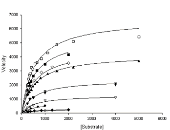
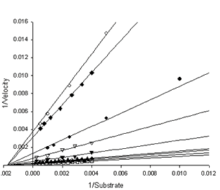
An excellent global fit is obtained to this data set. It is shown in the following Michaelis-Menten (Figure A) and Lineweaver-Burk (Figure B) graphs. The Km is 569 mM that can be seen to be a reasonable value for all curves in Figure A.


This example uses data sets that are column concatenated and index data values in a column of the worksheet. This isn’t necessary and the rabbit aorta concentration-response article shows how to write the curve fit equations to avoid column concatenation of the data. You may download a notebook with this data and enzyme kinetics fit object.
1. Duggleby, R.G. Pooling and Comparing Estimates from Several Experiments of a Michaelis Constant for an Enzyme, Anal. Biochem. 189 (1990), 84-87.
A global curve fit is the simultaneous fitting of multiple functions to multiple data sets with possible shared parameters.
|

